From last class
I emailed those who needed partner for their semester project.
Quiz: Go to kahoot.it
Linear models
A model is a linear model when the parameters enter linearly.
\(\mu_i = \beta_0 + x_i \beta_1 + x^2_i \beta_2\)
\(\mu_i = \beta_0 + x_{1i} \beta_1 + x_{2i}^{\beta_2}\)
\(\mu_i = \exp(x_{1i}\beta_1 + x_{2i}\beta_2)\)
The famous linear-plus-plateau model: \[\mu_i = \left \{
\begin{aligned}
& \beta_0 + x_i \beta_1 && \text{if } x_i \leq x_{crit}\\
& \beta_0 + x_{crit} \beta_1 && \text{if } x_i > x_{crit}
\end{aligned} \right.\]
Estimation
Continuous versus discrete independent variables.
How do we interpret them?
Recall the clover example :
3 clover species planted in pots.
24 plants per species.
After 2 months, we harvest and weigh their biomass.
We want to estimate how much biomass each genotype produces, eventually know how much and which one produces more.
library (tidyverse)<- read.csv ("data/lotus_part1.csv" ) %>% transmute (species = factor (species), agb_g) summary (dd_lotus)
 species     agb_g
 A:24    Min.   :1.265
 C:24    1st Qu.:1.969
 D:24    Median :2.355
         Mean   :2.492
         3rd Qu.:2.936
         Max.   :4.354
<- lm (agb_g ~ 0 + species, data = dd_lotus)
By programming m1 <- lm(agb_g ~ 0 + species, data = dd_lotus), we are fitting
\[\mathbf{y} \sim \text{N}(\boldsymbol{\mu}, \sigma^2\mathbf{I}),\] \[\boldsymbol{\mu}=\mathbf{X}\boldsymbol{\beta}.\]
What is another way of writing the model shown here?
Point estimates in \(\boldsymbol{\beta}\)
Let’s calculate \(\hat{\boldsymbol{\beta}}_{LSE} = (\mathbf{X}^T\mathbf{X})^{-1}\mathbf{X}^T\mathbf{y}\)
<- model.matrix (m1)<- dd_lotus$ agb_g<- solve (t (X)%*% X) %*% t (X)%*% y)
             [,1]
speciesA 2.936576
speciesC 2.396695
speciesD 2.143253
speciesA speciesC speciesD
2.936576 2.396695 2.143253
Residuals
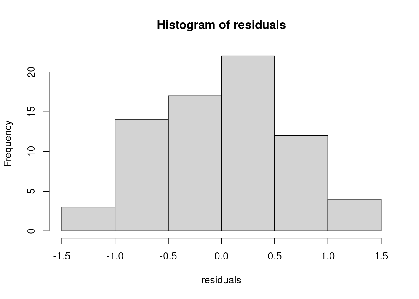
head (residuals <- y - X%*% beta_hat)
         [,1]
1 -0.02957583
2 -0.61733583
3 -0.21065583
4  0.47442417
5  1.29108417
6  0.25212417
        0%        25%        50%        75%       100%
-1.0413558 -0.4618581  0.0325275  0.4484598  1.4173242
          1           2           3           4           5           6
-0.02957583 -0.61733583 -0.21065583  0.47442417  1.29108417  0.25212417
        0%        25%        50%        75%       100%
-1.0413558 -0.4618581  0.0325275  0.4484598  1.4173242
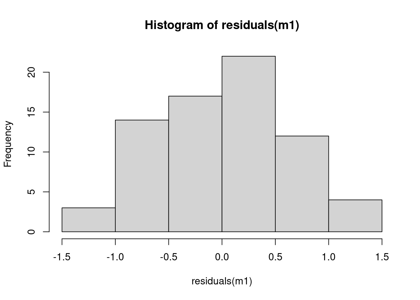
This will help us for model diagnostics (coming soon!)
Variance \(\sigma^2\)
Perhaps one of the most important parameters we will estimate.
Prediction accuracy.
Prediction intervals, estimation intervals.
Degrees of freedom. From \(n-1\) to \(n-p\) .
Let’s calculate \(\hat{\sigma}^2 = \frac{\boldsymbol{\hat{\varepsilon}^T\hat{\varepsilon}}}{n-p} = \frac{RSS}{n-p}\)
<- sum (residuals^ 2 )<- nrow (dd_lotus)<- length (beta_hat)<- RSS/ (n- p)) <- sqrt (sigma2_hat))
Confidence intervals
Confidence intervals are a measure of uncertainty. They are related to other measures of uncertainty, like \(\sigma^2\) . We know that \[CI = \hat{\beta} \pm t_{\alpha/2, dfe} \ s.e.,\] where \(t_{\alpha/2, dfe}\) is the t-score that corresponds to the confidence level (i.e., \(\alpha\) ) with the degrees of freedom of the error \(\text{rdf}\) , and \(s.e.\) is the standard error.
First, let’s calculate the standard error:
<- solve (t (X)%*% X)
<- sqrt (diag (unscaled_covariance))* sigma_hat)
speciesA speciesC speciesD
0.124231 0.124231 0.124231
<- 0.05 <- n- p<- qt (p= alpha/ 2 , df = dfe, lower.tail= F))
speciesA speciesC speciesD
0.247834 0.247834 0.247834
data.frame (lower = beta_hat - se* t_score, upper = beta_hat + se* t_score)
            lower    upper
speciesA 2.688742 3.184410
speciesC 2.148861 2.644529
speciesD 1.895419 2.391086
            2.5 %   97.5 %
speciesA 2.688742 3.184410
speciesC 2.148861 2.644529
speciesD 1.895419 2.391086
In summary:
Call:
lm(formula = agb_g ~ 0 + species, data = dd_lotus)

Residuals:
     Min       1Q   Median       3Q      Max
-1.04136 -0.46186  0.03253  0.44846  1.41732

Coefficients:
         Estimate Std. Error t value Pr(>|t|)
speciesA   2.9366     0.1242   23.64   <2e-16 ***
speciesC   2.3967     0.1242   19.29   <2e-16 ***
speciesD   2.1433     0.1242   17.25   <2e-16 ***
---
Signif. codes:  0 '***' 0.001 '**' 0.01 '*' 0.05 '.' 0.1 ' ' 1

Residual standard error: 0.6086 on 69 degrees of freedom
Multiple R-squared:  0.9468,    Adjusted R-squared:  0.9445
F-statistic: 409.5 on 3 and 69 DF,  p-value: < 2.2e-16
For next class
No reading!
Finish the assignment.
Schedule a meeting for the semester project.

