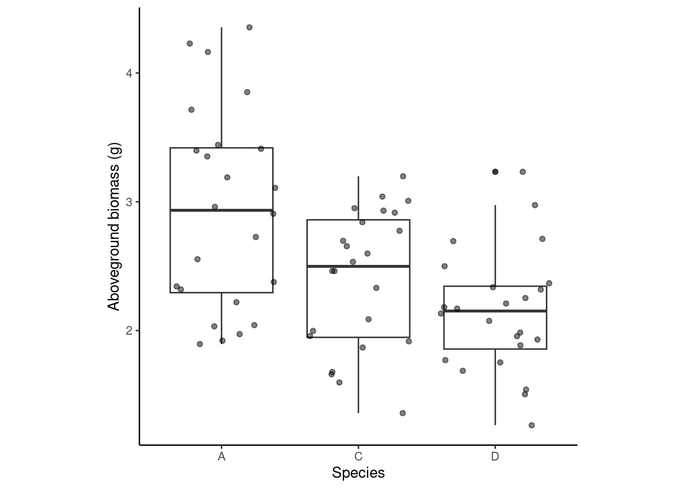
for \(i =1, 2, ..., n\), where \(n\) is the total number of observations, \(\mu_i\) is the mean of the \(i\)th observation, \(x_{1i}\), \(x_{2i}\), and \(x_{3i}\) are indicator variables that identify the species as A, C, or D, and thus \(\beta_1\), \(\beta_2\), and \(\beta_3\) are the means of genotypes A, C, and D, respectively, and \(\sigma^2\) is the variance of the data.
m <-lm(agb_g ~0+ species , data = data)
Define a bunch of objects needed for computations below:
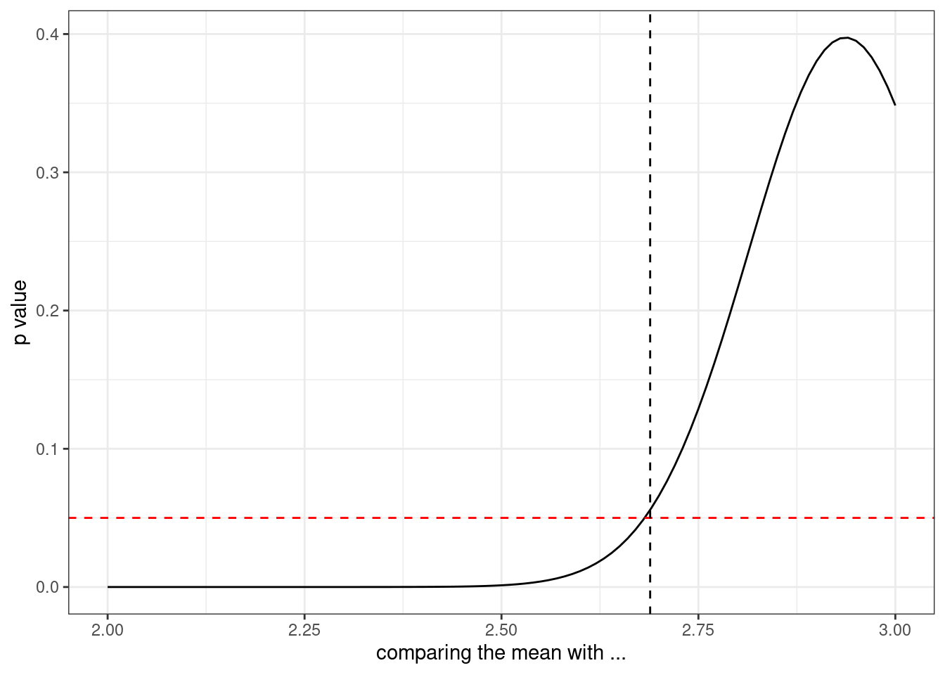
Recall that the t statistic \(T = \frac{\hat\theta}{s.e.(\hat\theta)}\) is used to compute the p value in hypothesis tests. We tested \(\beta_1 = 0\) before, but what about \(\beta_1 = \beta_2\)? In other words, we want to test if the difference between \(\beta_1\) and \(\beta_2\) is different to zero.
In this case, \(s.e.(\hat\beta_1 - \hat\beta_2) = \sqrt{s.e.(\hat\beta_1)^2+ s.e.(\hat\beta_2)^2 -2\text{cov}(\hat\beta_1, \hat\beta_2)}\).
comp <-seq(2, 3, by = .01)p.save <-numeric(length(comp))for (i in1:length(comp)) { p.save[i] <-dt((beta_hat[1] - comp[i])/( se[1]/sqrt(1)), dfe)}data.frame(comp, p.save) %>%ggplot(aes(comp, p.save))+geom_line()+labs(y ="p value", x ="comparing the mean with ...")+geom_hline(yintercept = .05, linetype =2, color ='red')+geom_vline(xintercept =confint(m)[1], linetype=2)+theme_bw()
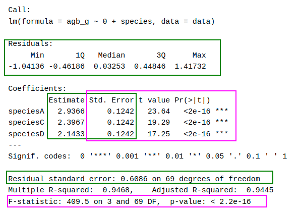
summary(m)
Call:
lm(formula = agb_g ~ 0 + species, data = data)

Residuals:
     Min       1Q   Median       3Q      Max
-1.04136 -0.46186  0.03253  0.44846  1.41732

Coefficients:
         Estimate Std. Error t value Pr(>|t|)
speciesA   2.9366     0.1242   23.64   <2e-16 ***
speciesC   2.3967     0.1242   19.29   <2e-16 ***
speciesD   2.1433     0.1242   17.25   <2e-16 ***
---
Signif. codes:  0 '***' 0.001 '**' 0.01 '*' 0.05 '.' 0.1 ' ' 1

Residual standard error: 0.6086 on 69 degrees of freedom
Multiple R-squared:  0.9468,    Adjusted R-squared:  0.9445
F-statistic: 409.5 on 3 and 69 DF,  p-value: < 2.2e-16
summary(lm(lm(agb_g ~ species , data = data)))
Call:
lm(formula = lm(agb_g ~ species, data = data))

Residuals:
     Min       1Q   Median       3Q      Max
-1.04136 -0.46186  0.03253  0.44846  1.41732

Coefficients:
            Estimate Std. Error t value Pr(>|t|)
(Intercept)   2.9366     0.1242  23.638  < 2e-16 ***
speciesC     -0.5399     0.1757  -3.073  0.00303 **
speciesD     -0.7933     0.1757  -4.515 2.54e-05 ***
---
Signif. codes:  0 '***' 0.001 '**' 0.01 '*' 0.05 '.' 0.1 ' ' 1

Residual standard error: 0.6086 on 69 degrees of freedom
Multiple R-squared:  0.2357,    Adjusted R-squared:  0.2135
F-statistic: 10.64 on 2 and 69 DF,  p-value: 9.399e-05
Summary
Now we know where (almost) everything in the summary output comes from!
summary(m)
But why do we care if something is significant?
The value in having categorized (“significant”/“non-significant” results)
What would you say for an effect with p = 0.049 and one with 0.051? Are both significant?
What is the difference between ‘significant’ and ‘non-significant’ results? See this paper.
A few things to have in mind when evaluating effects: