library(tidyverse)
library(ggpubr)
url <- "https://raw.githubusercontent.com/jlacasa/stat705_fall2024/main/classes/data/lotus_part4.csv"
dd <- read.csv(url)

dd_subset <- dd %>%
filter(trt == "ctrl")Day 15 - 09/23/2024
Analysis of Variance: ANOVA
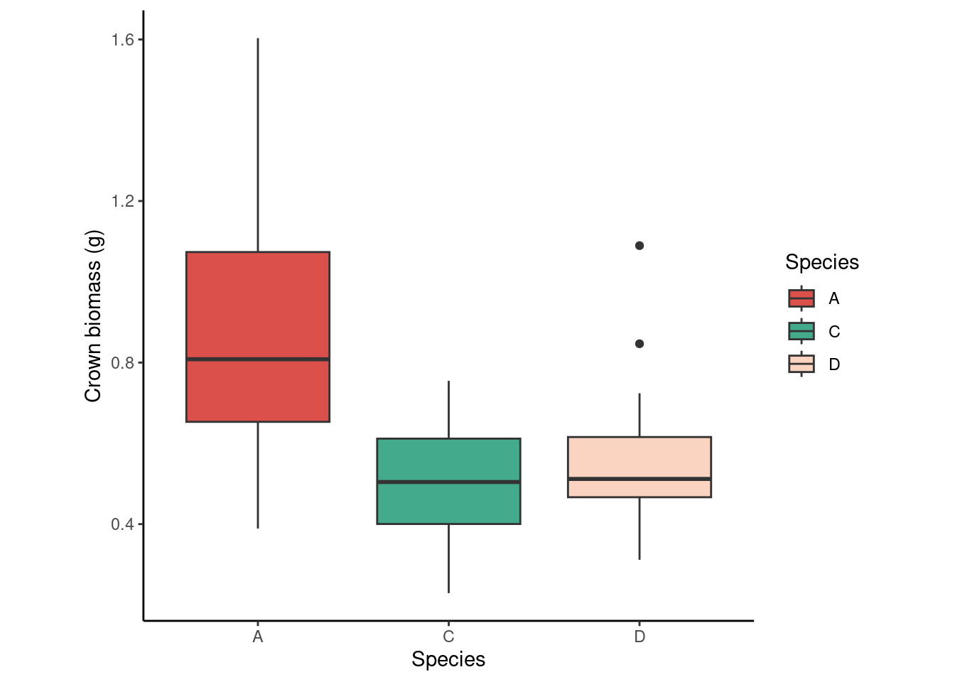
Helps us answering objectives like finding out “is A different to B or C?”, or “do any of these treatments have an effect on the mean?
Another types of objective (that require other types of modeling tools), for example, would be “to predict y for given levels of A and B” (e.g., predict corn yield with 150 kg N per ha and 20 inches rainfall in the season).
dd %>%
  ggplot(aes(species, crown_g))+
  geom_boxplot(aes(fill = species))+
  scale_fill_manual(values = c("#DB504A", "#43AA8B", "#FAD4C0"))+
  labs(x = "Species",
       y = "Crown biomass (g)",
       fill = "Species")+
  theme_classic()+
  theme(aspect.ratio = 1)
Let’s fit the model \[y_{ij} \sim N(\mu_{ij}, \sigma^2),\]
\[\mu_{ij} = \mu + \beta_{0j},\] where \(y_{ij}\) is the observation of crown biomass for the \(i\)th observation of the \(j\)th species, \(\mu{ij}\) is its mean and \(\sigma^2\) its variance. The means is described with the overall mean \(\mu\) and \(\beta_{0j}\), the effect of the \(j\)th species.
m1 <- lm(crown_g ~ species, data = dd_subset)
summary(m1)
Call:
lm(formula = crown_g ~ species, data = dd_subset)

Residuals:
     Min       1Q   Median       3Q      Max
-0.39175 -0.15785 -0.02829  0.15074  0.63792

Coefficients:
            Estimate Std. Error t value Pr(>|t|)
(Intercept)  0.96540    0.06631  14.560 6.36e-16 ***
speciesC    -0.49309    0.09377  -5.259 8.60e-06 ***
speciesD    -0.41107    0.09377  -4.384 0.000112 ***
---
Signif. codes:  0 '***' 0.001 '**' 0.01 '*' 0.05 '.' 0.1 ' ' 1

Residual standard error: 0.2297 on 33 degrees of freedom
Multiple R-squared:  0.4904,    Adjusted R-squared:  0.4595
F-statistic: 15.88 on 2 and 33 DF,  p-value: 1.477e-05
What’s another way of writing out this statistical model?
model.matrix(m1)[1:30,] (Intercept) speciesC speciesD
1 1 0 0
2 1 0 0
3 1 0 0
4 1 0 0
5 1 0 0
6 1 0 0
7 1 0 0
8 1 0 0
9 1 0 0
10 1 0 0
11 1 0 0
12 1 0 0
13 1 1 0
14 1 1 0
15 1 1 0
16 1 1 0
17 1 1 0
18 1 1 0
19 1 1 0
20 1 1 0
21 1 1 0
22 1 1 0
23 1 1 0
24 1 1 0
25 1 0 1
26 1 0 1
27 1 0 1
28 1 0 1
29 1 0 1
30 1 0 1One-way ANOVA
\[H_0: y_{ij} = \mu + \varepsilon_{ij}\] (\(H_0:\) All means are the same regardless of the predictor variable, indicated in subscript \(j\)).
\[H_1: y_{ij} = \mu + \beta_j + \varepsilon_{ij}\] (\(H_1:\) The means are different depending on the predictor variable, indicated in subscript \(j\)).
car::Anova(m1, type = "II")Anova Table (Type II tests)
Response: crown_g
Sum Sq Df F value Pr(>F)
species 1.6754 2 15.878 1.477e-05 ***
Residuals 1.7410 33
---
Signif. codes: 0 '***' 0.001 '**' 0.01 '*' 0.05 '.' 0.1 ' ' 1car::Anova(m1, type = "III")Anova Table (Type III tests)
Response: crown_g
Sum Sq Df F value Pr(>F)
(Intercept) 11.1841 1 211.990 6.360e-16 ***
species 1.6754 2 15.878 1.477e-05 ***
Residuals 1.7410 33
---
Signif. codes: 0 '***' 0.001 '**' 0.01 '*' 0.05 '.' 0.1 ' ' 1- Self-study questions:
- If the treatment factor has two levels, what is the difference between a t-test and an ANOVA test?
- Can you know which mean is larger based on the ANOVA results?
Two-way ANOVA
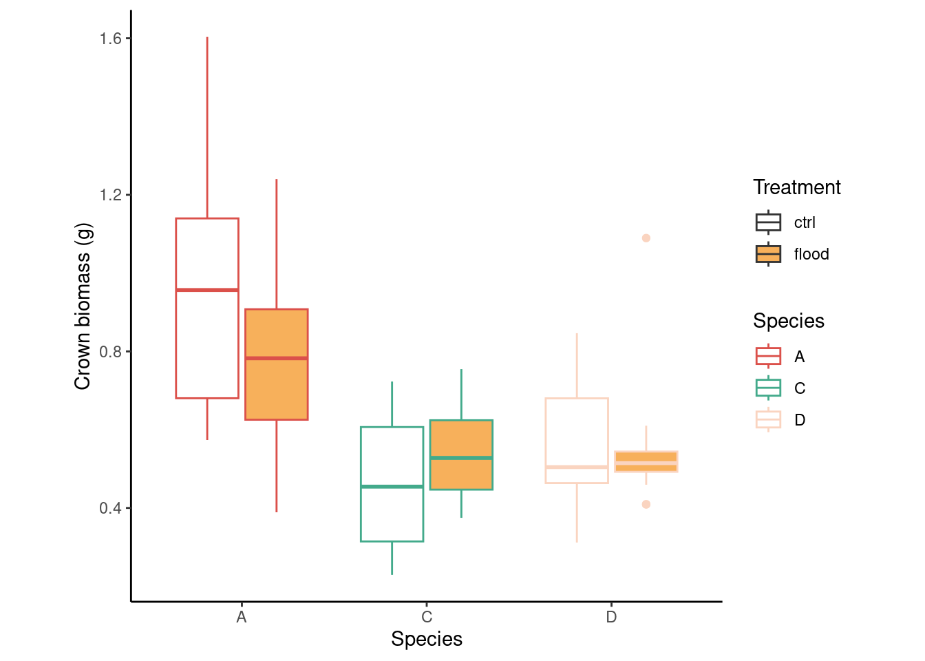
Used to answer the same types of questions, this analysis is most common in factorial designs.
dd %>%
  ggplot(aes(species, crown_g))+
  geom_boxplot(aes(fill = trt, color = species))+
  scale_fill_manual(values = c("white", "#F7B05B"))+
  scale_color_manual(values = c("#DB504A", "#43AA8B", "#FAD4C0"))+
  labs(x = "Species",
       y = "Crown biomass (g)",
       fill = "Treatment",
       color = "Species")+
  theme_classic()+
  theme(aspect.ratio = 1)
m2 <- lm(crown_g ~ species*trt, data = dd)
summary(m2)
Call:
lm(formula = crown_g ~ species * trt, data = dd)

Residuals:
     Min       1Q   Median       3Q      Max
-0.39578 -0.12946 -0.02559  0.12274  0.63791

Coefficients:
                  Estimate Std. Error t value Pr(>|t|)
(Intercept)        0.96541    0.06040  15.984  < 2e-16 ***
speciesC          -0.49310    0.08541  -5.773 2.28e-07 ***
speciesD          -0.41107    0.08541  -4.813 9.03e-06 ***
trtflood          -0.18065    0.08541  -2.115   0.0382 *
speciesC:trtflood  0.24622    0.12079   2.038   0.0455 *
speciesD:trtflood  0.17967    0.12079   1.487   0.1417
---
Signif. codes:  0 '***' 0.001 '**' 0.01 '*' 0.05 '.' 0.1 ' ' 1

Residual standard error: 0.2092 on 66 degrees of freedom
Multiple R-squared:  0.4279,    Adjusted R-squared:  0.3846
F-statistic: 9.875 on 5 and 66 DF, p-value: 4.427e-07model.matrix(m2)[1:30,] (Intercept) speciesC speciesD trtflood speciesC:trtflood speciesD:trtflood
1 1 0 0 0 0 0
2 1 0 0 0 0 0
3 1 0 0 0 0 0
4 1 0 0 0 0 0
5 1 0 0 0 0 0
6 1 0 0 0 0 0
7 1 0 0 0 0 0
8 1 0 0 0 0 0
9 1 0 0 0 0 0
10 1 0 0 0 0 0
11 1 0 0 0 0 0
12 1 0 0 0 0 0
13 1 1 0 0 0 0
14 1 1 0 0 0 0
15 1 1 0 0 0 0
16 1 1 0 0 0 0
17 1 1 0 0 0 0
18 1 1 0 0 0 0
19 1 1 0 0 0 0
20 1 1 0 0 0 0
21 1 1 0 0 0 0
22 1 1 0 0 0 0
23 1 1 0 0 0 0
24 1 1 0 0 0 0
25 1 0 1 0 0 0
26 1 0 1 0 0 0
27 1 0 1 0 0 0
28 1 0 1 0 0 0
29 1 0 1 0 0 0
30 1 0 1 0 0 0car::Anova(m2, type = "II")Anova Table (Type II tests)
Response: crown_g
Sum Sq Df F value Pr(>F)
species 1.93969 2 22.1558 4.35e-08 ***
trt 0.02694 1 0.6154 0.4356
species:trt 0.19466 2 2.2235 0.1163
Residuals 2.88908 66
---
Signif. codes: 0 '***' 0.001 '**' 0.01 '*' 0.05 '.' 0.1 ' ' 1car::Anova(m2, type = "III")Anova Table (Type III tests)
Response: crown_g
Sum Sq Df F value Pr(>F)
(Intercept) 11.1841 1 255.4967 < 2.2e-16 ***
species 1.6754 2 19.1370 2.787e-07 ***
trt 0.1958 1 4.4729 0.03822 *
species:trt 0.1947 2 2.2235 0.11628
Residuals 2.8891 66
---
Signif. codes: 0 '***' 0.001 '**' 0.01 '*' 0.05 '.' 0.1 ' ' 1Using a combination of categorical (indicator) variables and continuous variables
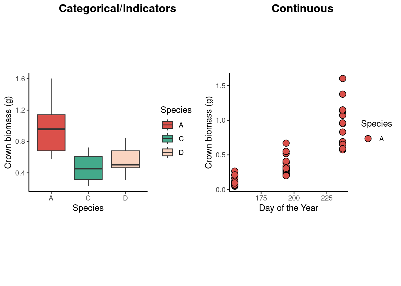
Review types of explanatory data
url2 <- "https://raw.githubusercontent.com/jlacasa/stat705_fall2024/main/classes/data/lotus_part3.csv"
dd2 <- read.csv(url2)
ggarrange(
 dd2 %>%
   filter(doy ==237) %>%
    ggplot(aes(species, crown_g))+
    geom_boxplot(aes(fill = species))+
    scale_fill_manual(values = c("#DB504A", "#43AA8B", "#FAD4C0"))+
    labs(x = "Species",
         y = "Crown biomass (g)",
         fill = "Species")+
    theme_classic()+
    theme(aspect.ratio = 1),
 dd2 %>%
   filter(species== "A") %>%
   ggplot(aes(doy, crown_g))+
    geom_point(aes(fill = species), shape = 21, size =3.5)+
    scale_fill_manual(values = c("#DB504A", "#43AA8B", "#FAD4C0"))+
    labs(x = "Day of the Year",
         y = "Crown biomass (g)",
         fill = "Species")+
    theme_classic()+
    theme(aspect.ratio = 1),
 ncol =2,
 labels = c("Categorical/Indicators", "Continuous"),
 label.x = c(0, 0.2)
)
dd2 %>%
  ggplot(aes(doy, crown_g))+
  geom_point(aes(fill = species), shape = 21, size =3.5)+
  scale_fill_manual(values = c("#DB504A", "#43AA8B", "#FAD4C0"))+
  labs(x = "Day of the Year",
       y = "Crown biomass (g)",
       fill = "Species")+
  theme_classic()+
  theme(aspect.ratio = 1)
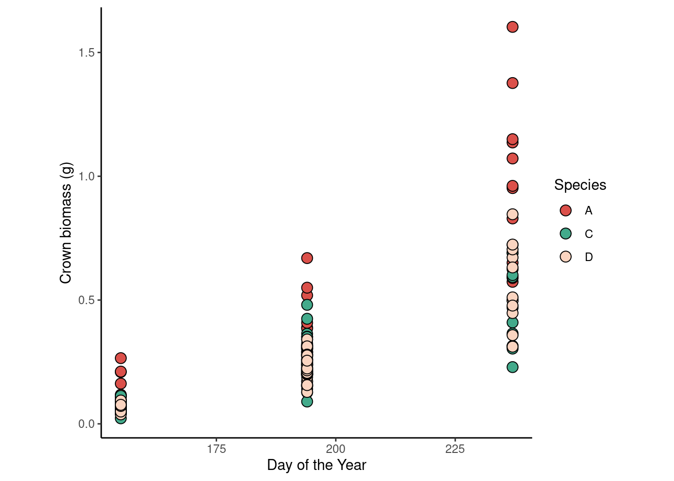
m3 <- lm(crown_g ~ species*doy, data = dd2)

summary(m3)
Call:
lm(formula = crown_g ~ species * doy, data = dd2)

Residuals:
     Min       1Q   Median       3Q      Max
-0.29416 -0.09688 -0.00858  0.06046  0.73550

Coefficients:
               Estimate Std. Error t value Pr(>|t|)
(Intercept)  -1.5809069  0.1438577 -10.989  < 2e-16 ***
speciesC      0.8764868  0.2034455   4.308 3.11e-05 ***
speciesD      0.6864100  0.2034455   3.374 0.000962 ***
doy           0.0103322  0.0007297  14.159  < 2e-16 ***
speciesC:doy -0.0054042  0.0010320  -5.237 5.96e-07 ***
speciesD:doy -0.0043320  0.0010320  -4.198 4.80e-05 ***
---
Signif. codes:  0 '***' 0.001 '**' 0.01 '*' 0.05 '.' 0.1 ' ' 1

Residual standard error: 0.1467 on 138 degrees of freedom
Multiple R-squared:  0.7207,    Adjusted R-squared:  0.7105
F-statistic: 71.21 on 5 and 138 DF, p-value: < 2.2e-16car::Anova(m3, type = "III")Anova Table (Type III tests)
Response: crown_g
Sum Sq Df F value Pr(>F)
(Intercept) 2.5974 1 120.766 < 2.2e-16 ***
species 0.4419 2 10.272 6.937e-05 ***
doy 4.3120 1 200.491 < 2.2e-16 ***
species:doy 0.6614 2 15.376 9.368e-07 ***
Residuals 2.9680 138
---
Signif. codes: 0 '***' 0.001 '**' 0.01 '*' 0.05 '.' 0.1 ' ' 1model.matrix(m3)[1:30,] (Intercept) speciesC speciesD doy speciesC:doy speciesD:doy
1 1 0 0 155 0 0
2 1 0 0 155 0 0
3 1 0 0 155 0 0
4 1 0 0 155 0 0
5 1 0 0 155 0 0
6 1 0 0 155 0 0
7 1 0 0 155 0 0
8 1 0 0 155 0 0
9 1 0 0 155 0 0
10 1 0 0 155 0 0
11 1 0 0 155 0 0
12 1 0 0 155 0 0
13 1 1 0 155 155 0
14 1 1 0 155 155 0
15 1 1 0 155 155 0
16 1 1 0 155 155 0
17 1 1 0 155 155 0
18 1 1 0 155 155 0
19 1 1 0 155 155 0
20 1 1 0 155 155 0
21 1 1 0 155 155 0
22 1 1 0 155 155 0
23 1 1 0 155 155 0
24 1 1 0 155 155 0
25 1 0 1 155 0 155
26 1 0 1 155 0 155
27 1 0 1 155 0 155
28 1 0 1 155 0 155
29 1 0 1 155 0 155
30 1 0 1 155 0 155Let’s put this in context
- Don’t forget our assumptions:
- residuals are iid \(\sim N(0, \sigma^2)\)
- parameters enter linearly (linear model)
- homoscedasticity (i.e., constant variance)
- residuals are iid \(\sim N(0, \sigma^2)\)
- Whiteboard. Context in data analysis workflow.
For next class
- Read Chapter 15.
- Resubmit Assignment 2.
- Following: model diagnostics, model selection.