Day 21 - 10/07/2024

Announcements

Model selection

Recall the conceptual pipeline we use to solve our problems using statistics.
1. Idea/Question/Objective
2. Gathering data
3. Building a statistical model (i.e., assumptions about the data generating process)
4. Fitting the model to data
5. Model diagnostics
6. Model selection
7. Inference
8. Communicating results
Sometimes, there exists a group of models that could possibly answer our question in (1) and make relatively reasonable assumptions (i.e., they pass the test in (2)). So, we have to select between this group of models which one is the best.
How many variables should we include?
- Bias-variance trade off
We have to define what “good” means!
- Penalized fit (i.e., penalty for including too many parameters)
  - Information Criteria (e.g., AIC, BIC)
  - R²_adj
- Out-of-sample prediction accuracy
  - Cross-validation
  - RMSEP (prediction root mean squared error)
- A paper on how to evaluate predictions versus observed values.

Applications

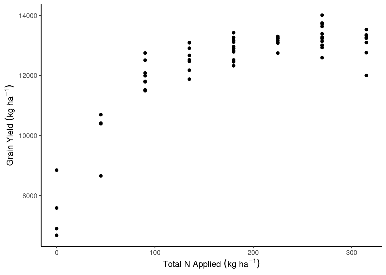
Using the data from Ransom et al. (2021), we wish to create a function that describes the relationship between Nitrogen supply and corn yield. Firstly, we will focus on a single site and year (Ames, IA, 2014).

Load the data

library(tidyverse)

# find data at https://doi.org/10.1002/agj2.20812
dd_yield <- readxl::read_xlsx("data/8.Yield_Plant_Measurements.xlsx", sheet = 2) %>%
  filter(Year == 2014, 
         State == "IA", 
         Site == "Ames") %>% 
  mutate(across(VT_TissN:R4N, ~ as.numeric(.)))
dd_soil <- readxl::read_xlsx("data/1.Site_Characterization.xlsx", sheet = 2) %>% 
  filter(Year == 2014, 
         State == "IA", 
         Site == "Ames", 
         Horizon == "Ap") %>% 
  mutate(Block = as.numeric(Block), 
         across(Clay:WC, ~as.numeric(.)))
dd_N <- readxl::read_xlsx("data/4.SoilN.xlsx", sheet = 2) %>% 
  filter(Year == 2014, 
         State == "IA", 
         Site == "Ames", 
         Plot_ID %in% dd_yield$Plot_ID, 
         Sam_Time == "Post") %>% 
  mutate(across(c(Plot_ID, N_Trt, Plant_N, Side_N, Plant_N_SI, Side_N_SI), ~as.numeric(.)))

dd_complete <- dd_yield %>% 
  left_join(dd_soil) %>% 
  left_join(dd_N)

dd_complete <- dd_complete %>% 
  mutate(gyield_14 = GYdry/.94, 
         N_total = Plant_N_SI + Side_N_SI)

dd_complete %>% 
  ggplot(aes(N_total, gyield_14))+
  geom_point()+
  theme_classic()+
  labs(x = expression(Total~N~Applied~(kg~ha^{-1})),
       y = expression(Grain~Yield~(kg~ha^{-1})))

Fit the to some models

m0 <- lm(gyield_14 ~ N_total, data = dd_complete)
m1 <- lm(gyield_14 ~ N_total + I(N_total^2), data = dd_complete)
m2 <- lm(gyield_14 ~ N_total + I(N_total^2) + Block , data = dd_complete)
m3 <- lm(gyield_14 ~ N_total + I(N_total^2) + Block + PMPM, data = dd_complete)
m4 <- lm(gyield_14 ~ N_total + I(N_total^2) + Block + PMPM + Clay, data = dd_complete)   
m5 <- lm(gyield_14 ~ N_total + I(N_total^2) + Block + PMPM + Clay + Sand, data = dd_complete)
m6 <- lm(gyield_14 ~ N_total + I(N_total^2) + Block + PMPM + Clay + Sand + Silt, data = dd_complete)

n <- nobs(m1)

Select the best models

AIC

\[AIC_M = 2p - 2\log(\hat{L}),\]

p <- length(coef(m1))+1
log_lik <- -n / 2 * (log(2 * pi) + log(sum(m1$residuals^2) / n) + 1)
2*p - 2*log_lik

[1] 997.5004

AIC(m1)

[1] 997.5004

BIC

\[BIC_M = p \cdot log(n) - 2\log(\hat{L}),\]

# for BIC, k is log(nobs(m1))
log(nobs(m1))*p - 2*log_lik

[1] 1006.136

AIC(m1, k = log(nobs(m1)))

[1] 1006.136

BIC(m1)

[1] 1006.136

R² and R²_adj

Recall that
\[R^2 = 1-\frac{SSE}{SST}\] is considered the proportion of variation in y explained by variation in x (or in my model, if I have more than one predictor).
R², however, does not penalize for adding more predictors (i.e., more parameters) and can only increase. We solve this by calculating

\[R^2_{adj} = R^2 - (1 - R^2) \frac{p-1}{n-p},\] where \(n\) is the number of observations and \(p\) is the number of parameters.

Downfalls of using R² for model selection

Uncertainty (precision is tricky with small sample size)
Using the same data twice (once to fit the models, then to judge the models!)
Anscombe’s quartet

A summary

summary(m5)


Call:
lm(formula = gyield_14 ~ N_total + I(N_total^2) + Block + PMPM + 
    Clay + Sand, data = dd_complete)

Residuals:
     Min       1Q   Median       3Q      Max 
-1358.67  -369.15    50.32   395.71  1328.61 

Coefficients:
               Estimate Std. Error t value Pr(>|t|)    
(Intercept)  -1.785e+04  2.108e+04  -0.847    0.401    
N_total       4.556e+01  2.838e+00  16.052   <2e-16 ***
I(N_total^2) -9.704e-02  8.118e-03 -11.955   <2e-16 ***
Block         4.780e+02  3.068e+02   1.558    0.125    
PMPM          1.999e+01  1.962e+01   1.019    0.313    
Clay          6.088e+02  5.213e+02   1.168    0.248    
Sand          2.290e+02  2.007e+02   1.141    0.259    
---
Signif. codes:  0 '***' 0.001 '**' 0.01 '*' 0.05 '.' 0.1 ' ' 1

Residual standard error: 554.9 on 57 degrees of freedom
Multiple R-squared:  0.8856,    Adjusted R-squared:  0.8736 
F-statistic: 73.55 on 6 and 57 DF,  p-value: < 2.2e-16

summary(m6)


Call:
lm(formula = gyield_14 ~ N_total + I(N_total^2) + Block + PMPM + 
    Clay + Sand + Silt, data = dd_complete)

Residuals:
     Min       1Q   Median       3Q      Max 
-1358.67  -369.15    50.32   395.71  1328.61 

Coefficients: (1 not defined because of singularities)
               Estimate Std. Error t value Pr(>|t|)    
(Intercept)  -1.785e+04  2.108e+04  -0.847    0.401    
N_total       4.556e+01  2.838e+00  16.052   <2e-16 ***
I(N_total^2) -9.704e-02  8.118e-03 -11.955   <2e-16 ***
Block         4.780e+02  3.068e+02   1.558    0.125    
PMPM          1.999e+01  1.962e+01   1.019    0.313    
Clay          6.088e+02  5.213e+02   1.168    0.248    
Sand          2.290e+02  2.007e+02   1.141    0.259    
Silt                 NA         NA      NA       NA    
---
Signif. codes:  0 '***' 0.001 '**' 0.01 '*' 0.05 '.' 0.1 ' ' 1

Residual standard error: 554.9 on 57 degrees of freedom
Multiple R-squared:  0.8856,    Adjusted R-squared:  0.8736 
F-statistic: 73.55 on 6 and 57 DF,  p-value: < 2.2e-16

metrics <- data.frame(model = c("N_total", 
                                "N_total + I(N_total^2)",
                                "N_total + I(N_total^2) + Block",
                                "N_total + I(N_total^2) + Block + PMPM", 
                                "N_total + I(N_total^2) + Block + PMPM + Clay", 
                                "N_total + I(N_total^2) + Block + PMPM + Clay + Sand", 
                                "N_total + I(N_total^2) + Block + PMPM + Clay + Sand + Silt"),
                      R2 = c(summary(m0)$r.squared, summary(m1)$r.squared, summary(m2)$r.squared, 
                             summary(m3)$r.squared, summary(m4)$r.squared, summary(m5)$r.squared, summary(m6)$r.squared),
                      R2_adj = c(summary(m0)$adj.r.squared, summary(m1)$adj.r.squared, summary(m2)$adj.r.squared,
                                 summary(m3)$adj.r.squared, summary(m4)$adj.r.squared, summary(m5)$adj.r.squared,
                                 summary(m6)$adj.r.squared),
                      AIC = AIC(m0, m1, m2, m3, m4, m5, m6)$AIC,
                      BIC = BIC(m0, m1, m2, m3, m4, m5, m6)$BIC) %>% 
  mutate(across(R2:BIC, ~round(., 3)))

knitr::kable(metrics, format = "html")

model	R2	R2_adj	AIC	BIC
N_total	0.589	0.582	1070.935	1077.412
N_total + I(N_total^2)	0.873	0.869	997.500	1006.136
N_total + I(N_total^2) + Block	0.878	0.872	997.147	1007.941
N_total + I(N_total^2) + Block + PMPM	0.882	0.874	996.822	1009.775
N_total + I(N_total^2) + Block + PMPM + Clay	0.883	0.873	998.453	1013.566
N_total + I(N_total^2) + Block + PMPM + Clay + Sand	0.886	0.874	999.008	1016.279
N_total + I(N_total^2) + Block + PMPM + Clay + Sand + Silt	0.886	0.874	999.008	1016.279

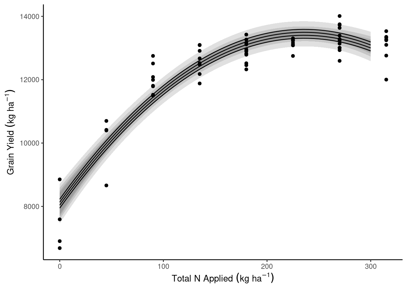
data_plot <- expand.grid(N_total = seq(0, 300, by = 5), 
                         Block = 1:4)
data_plot <- data_plot %>% bind_cols(predict(m2, newdata = data_plot, interval = "confidence"))

dd_complete %>% 
  ggplot(aes(N_total, gyield_14))+
  theme_classic()+
  geom_ribbon(aes(y = fit, ymin = lwr, ymax = upr, group = Block), data = data_plot, alpha = .15)+
  geom_line(aes(y = fit, group = Block), data = data_plot)+
  geom_point()+
  labs(x = expression(Total~N~Applied~(kg~ha^{-1})),
       y = expression(Grain~Yield~(kg~ha^{-1})))

A question for the class

How do you expect the variable selection to change if we add more…

sites
years

Important questions/concepts

Variable selection - checkpoints

How do the predictions compare?
Is the data generation process well represented?
What is the cost/benefit relationship of including certain predictors?

Watch out with

Collinearity
Using the same data twice (once to fit the models, then to judge the models!)

For next class

Read Chapter 8 & 10
Finish Assignment 3