Simulation example for day 5 - 08/28/2024

Set the parameters

## 'true' parameters
beta0_truth <- 5
beta1_truth <- .25
sigma2_truth <- 15

## data
x <- seq(1000, 1200, length.out = 60)
mu <- beta0_truth + x*beta1_truth 
n <- length(x) # total number of observations
set.seed(3298)
epsilon <- rnorm(n, 0, sqrt(sigma2_truth)) # error

# observed data
y <- mu + epsilon

plot(x, y)
points(x, mu, ty = 'l', col = 'red')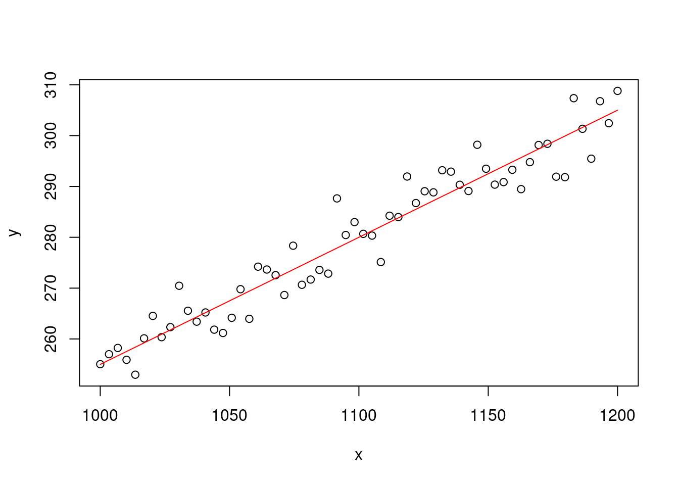

simulated_data <- data.frame(x= x, y=y)

m1 <- lm(y ~ 1 + x, data = simulated_data)

coef(m1)

(Intercept)           x 
  8.5594283   0.2467447 

confint(m1)

                  2.5 %     97.5 %
(Intercept) -11.0441489 28.1630056
x             0.2289486  0.2645408

#setting nr of simulations
n_sims <- 1000
# creating the pace to store
intercept <- numeric(length = n_sims)
slope <- numeric(length = n_sims)
sigma <- numeric(length = n_sims)

for (i in 1:n_sims){
  e <- rnorm(n, 0, sqrt(sigma2_truth))
  y <- mu + e
  simulated_data <- data.frame(x= x, y=y)
  m1 <- lm(y ~ 1 + x, data = simulated_data)
  intercept[i] <- coef(m1)[1]
  slope[i] <- coef(m1)[2]
  sigma[i] <- summary(m1)$sigma
}

data.frame(slope) %>% 
  ggplot(aes(x = slope))+
  geom_histogram()+
  geom_vline(linetype =2, col = "gold", xintercept = beta1_truth)+
  labs(x = TeX("$\\beta_1$"))+
  theme_bw()+
  theme(aspect.ratio = 1)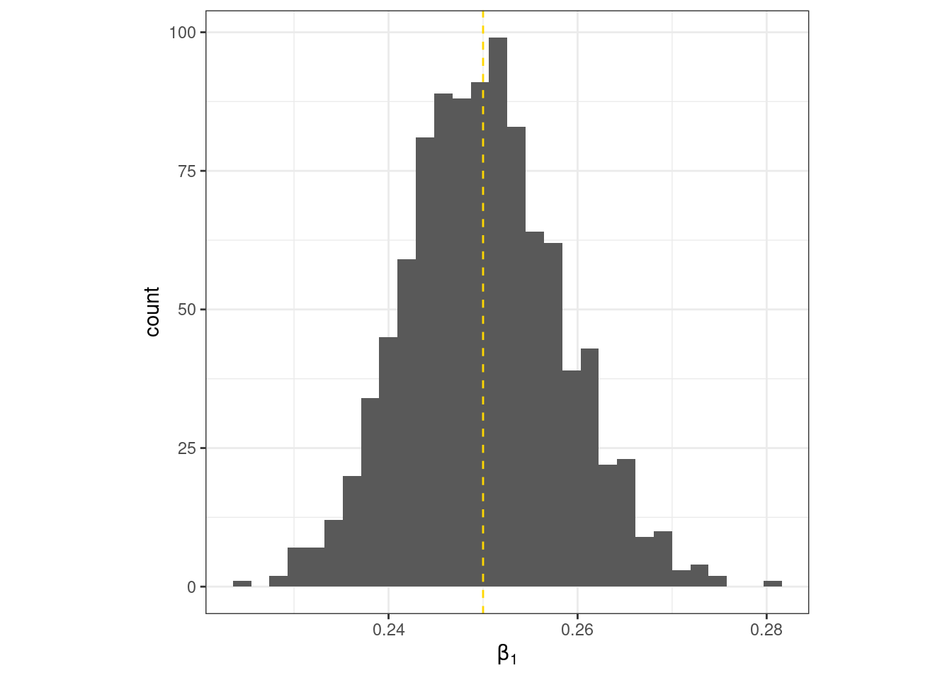

data.frame(sigma) %>% 
  ggplot(aes(x = sigma^2))+
  geom_histogram()+
  geom_vline(linetype =2, col = "gold", xintercept = sigma2_truth)+
  labs(x = TeX("$\\sigma^2$"))+
  theme_bw()+
  theme(aspect.ratio = 1)

data.frame(slope, intercept) %>% 
  ggplot(aes(x = slope, y = intercept))+
  geom_point()+
  labs(x = TeX("$\\beta_1$"), 
       y = TeX("$\\beta_0$"))+
  theme_bw()+
  theme(aspect.ratio = 1)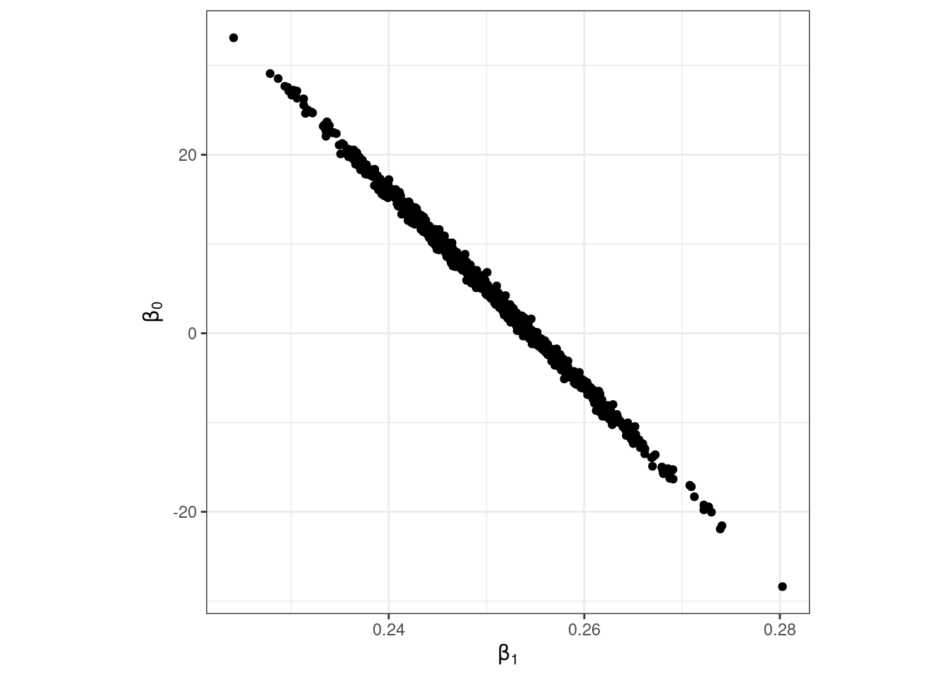

beta1_truth

[1] 0.25

mean(slope)

[1] 0.2500702

sigma2_truth

[1] 15

mean(sigma^2)

[1] 15.04852