From last class
Fill out this form if you need a project partner.
Back to our clover example.
The General Linear Model
When we fit models using the lm function, we are fitting a general linear model. We can express our model as:
\[y_i \sim \text{N}(\mu_i, \sigma^2),\]
\[\mu_i = z_{1 i}\cdot \beta{1} + z_{2 i}\cdot \beta_2 + z_{3 i}\cdot \beta_3,\]
\[z_{1 i} \left \{
\begin{aligned}
& 1 && \text{if species A} \\
& 0 && \text{else}
\end{aligned} \right.,\]
\[z_{2 i} \left \{
\begin{aligned}
& 1 && \text{if species B} \\
& 0 && \text{else}
\end{aligned} \right.,\]
\[z_{3 i} \left \{
\begin{aligned}
& 1 && \text{if species C} \\
& 0 && \text{else}
\end{aligned} \right.,\]
for \(i = 1, 2, ... n\) where \(n\) is the total number of observations. Our data can only be A, or C, or D. So that basically gives us rows of 1s and 0s.
Recall that our design matrix looked very much like
\[\mathbf{X}=
\left(
\matrix{0 & 0 & 1 \\
0 & 1 & 0 \\
1 & 0 & 0 \\
0 & 1 & 0 \\
1 & 0 & 0 \\
0 & 0 & 1}
\right).\]
In this case, the matrix has 6 rows, so \(n=6\) .
We are assuming:
Linearity
Homoscedasticity
Independence
Normality
Another linear model example
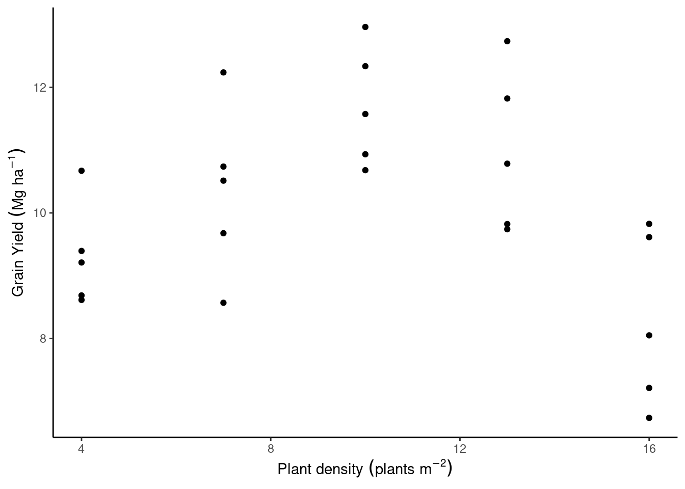
<- "https://raw.githubusercontent.com/jlacasa/stat705_fall2024/main/classes/data/corn_example1.csv" <- read.csv (url)head (data)
  plant_density rep yield_Mgha
1             4   1   8.685132
2             7   1   9.676261
3            10   1  12.336717
4            13   1  10.783971
5            16   1   9.613427
6             4   2   9.393913
library (tidyverse)%>% ggplot (aes (plant_density, yield_Mgha))+ geom_point ()+ theme_classic ()+ labs (x = expression (Plant~ density~ (plants~ m^ {- 2 })), y = expression (Grain~ Yield~ (Mg~ ha^ {- 1 })))
Let’s write out the statistical model:
\[y_i \sim \text{N}(\mu_i, \sigma^2),\]
\[\mu_i = \beta_0 + \beta_1\cdot x_i + \beta_2 \cdot x_i^2.\]
Live R code example to fit this model to the data here .
Estimation
The method we are using in lm is called Maximum Likelihood Estimation.
Least Squares estimation (LSE) versus Maximum Likelihood estimation (MLE)
LSE minimizes \(\Sigma_{i=1}^n \varepsilon_i^2\) , where \(\varepsilon_i = y_i-\mu_i\) .
That gives us \(\hat{\boldsymbol{\beta}} = (\mathbf{X}^T\mathbf{X})^{-1}\mathbf{X}^T\mathbf{y}\) .
If the errors are independent and identically normally distributed, \(\hat{\boldsymbol{\beta}}_{LSE} = \hat{\boldsymbol{\beta}}_{MLE}\) .
what does “independent and identically normally distributed” mean?
\(\hat{\boldsymbol{\beta}}\) is the best linear unbiased estimator!
Estimation - an applied example
Live R session.
General notation
\[\mathbf{y} \sim \text{N}(\boldsymbol{\mu}, \sigma^2\mathbf{I}),\]
\[\boldsymbol{\mu} = \mathbf{X}\boldsymbol{\beta},\]
where \(\mathbf{y}\) are the observed data, \(\boldsymbol{\mu}\) is the expected value, \(\sigma^2\) is the variance, \(\mathbf{X}\) is the design matrix, and \(\boldsymbol{\beta}\) is a vector of parameters.
This notation is convenient to think about the data for your project. One row per observation (rows in \(\mathbf{X}\) ), one variable per column (columns in \(\mathbf{X}\) ).
For next week
Read chapter 3 from the book.
Remember Assignment 1 is on.
Heads up, in-class quiz for attendance.
