3 TAPS - some learning
3.1 What is special about TAPS designs?
Designed experiments in TAPS are typically arranged in a randomized complete block design (RCBD).
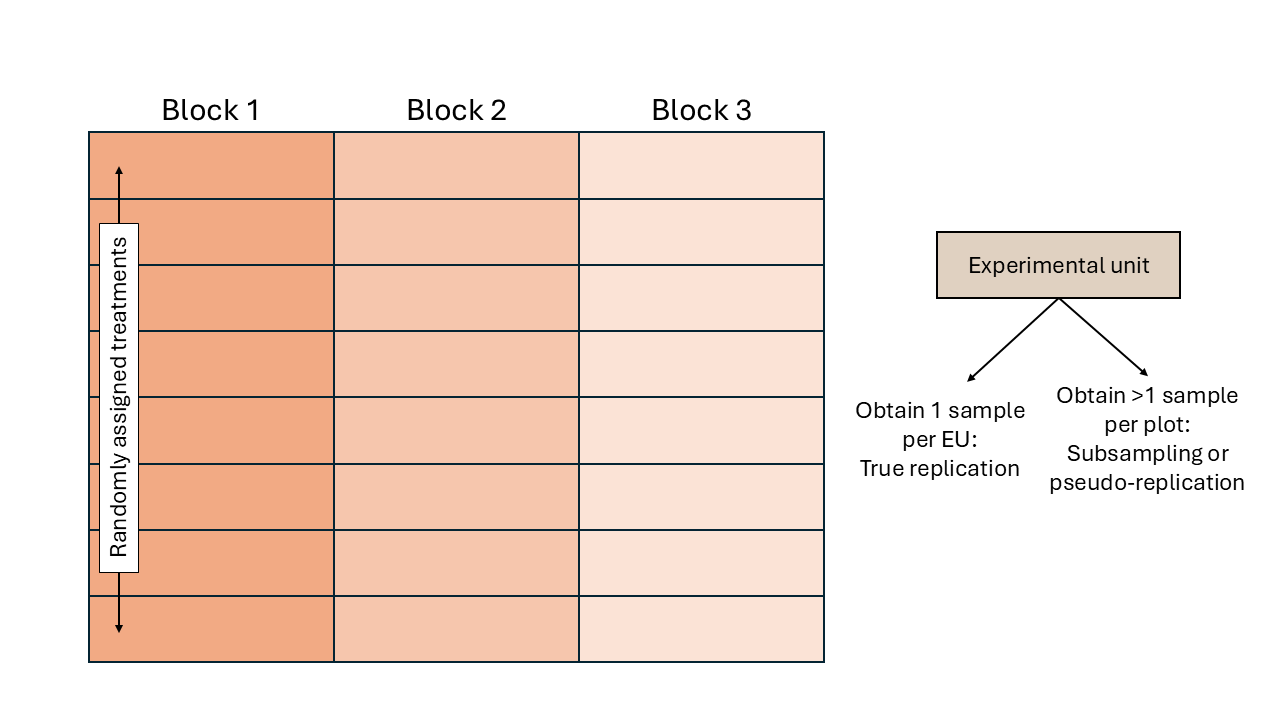
Figure 3.1: Schematic representation of a randomized complete block design.
Some TAPS designed experiments are arranged in a split-plot design.
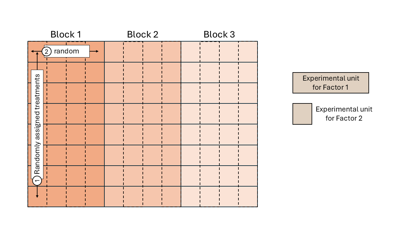
Figure 3.2: Schematic representation of a split-plot design randomized complete block arrangement.
- Designs are D-Optimal - best to estimate the team’s yield/profit precisely.
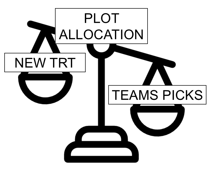
Figure 3.3: Prioritizing our research questions often seems like a balancing act between resources allocated to the competition, and resources allocated to additional research.
3.2 An applied example
A manager is designing a competition with 24 teams signed up, and needs to decide whether to use 4 replicates or 3 replicates and allocate more resources to the research question.
Some questions:
- What is the trade-off between #reps and #points?
- How do we assign the new treatments?
Consider the following options:
| # Teams | # Reps per team | # Plots assigned to other treatments | Total plots available |
|---|---|---|---|
| 24 | 4 | 12 + 48 | 108 |
| 24 | 3 | 12 + 24 | 108 |
| 24 | 2 | 12 | 108 |
Mathematically, we can infer a few points:
- Recall that \(se(\hat{\mu_j}) =\sqrt\frac{\sigma^2}{r}\).
| # Teams | # Reps per team | # Plots assigned to other treatments | SE(Teams mean) |
|---|---|---|---|
| 24 | 4 | 12 + 48 | sigma2/sqrt(4) = 0.5 sigma |
| 24 | 3 | 12 + 24 | sigma2/sqrt(3) = 0.58 sigma |
| 24 | 2 | 12 | sigma2/sqrt(2) = 0.71 sigma |
How are the estimates of N and Irr affected?
- Recall that \(se(\hat{\boldsymbol\beta}) =\sqrt{\sigma^2 (\mathbf{X}^\top\mathbf{X})^{-1}}\) and thus \(se(\hat{\beta_j}) =\sqrt{\sigma^2 (\mathbf{X}^\top\mathbf{X})^{-1}_{jj}}\).
Essentially,
\[se(\hat\beta_j) = \sqrt{\sigma^2 (r\mathbf{X}_{teams}^\top \mathbf{X}_{teams} + \mathbf{X}_{extra}^\top \mathbf{X}_{extra})^{-1}}\]
We can also consider different \(\sigma^2\) for treatment versus extra.
\[se(\hat\beta_j) = \sqrt{(\frac{1}{\sigma^2_t} r\mathbf{X}_{teams}^\top \mathbf{X}_{teams} + \frac{1}{\sigma^2_{extra}} \mathbf{X}_{extra}^\top \mathbf{X}_{extra})^{-1}_{jj}}\]
3.2.1 Comparing designs side by side
| # reps | Extra plots | SE(trt mean) | SE(Intercept) | SE(N) | SE(Irr) | SE(N^2) | SE(Irr^2) | SE(NxIrr) | SE(OPT N) | SE(OPT Irr) | |
|---|---|---|---|---|---|---|---|---|---|---|---|
| Option 1 | 4 | 0 | 30.000 | 126.996 | 1.881 | 30.585 | 0.009 | 1.572 | 0.252 | 20.201 | 1.441 |
| Option 2 | 4 | 12 | 30.000 | 115.235 | 1.185 | 14.039 | 0.004 | 0.652 | 0.072 | 14.010 | 0.987 |
| Option 3 | 3 | 36 | 34.641 | 109.026 | 1.003 | 12.986 | 0.003 | 0.560 | 0.045 | 12.677 | 0.879 |
| Option 4 | 2 | 60 | 42.426 | 108.776 | 0.969 | 12.882 | 0.003 | 0.555 | 0.041 | 12.294 | 0.768 |
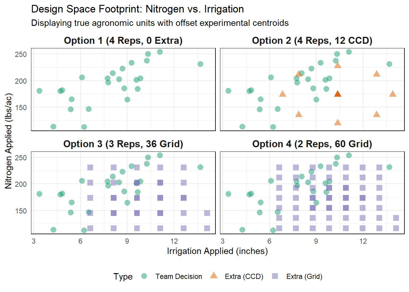
Figure 3.4: Design spaces in raw units. Collinear team behavior is shown alongside the extra treatments offset to map unexplored regions.